Filters - An introduction

02 Oct, 2025

--Sections--

Low-Pass Filters(LPF)
RC LPF Theory
RC LPF Analysis
RC LPF Frequency Response
Capacitors
Visualizing Noise Filtering
Internal link

Introduction

I began working as a Teaching Assistant a little over a year now. Having taught circuit courses, I've seen students struggle with various aspects of these classes' labs. A specific difficulty that I seem to encounter almost all TA sessions is that of noise and by association filtering.

When working with noisy power supplies, non ideal function generators, and cheap IC components, it's an inevitability that students will face problems that inhibit their ability to finish labs.

In all of the circuit course labs I've encountered, the signal frequencies that we use are quite low(less than 10kHz) and the type of noise usually encountered is white.

Let's quickly define white noise. "Noise" refers to any unwanted signal or disturbance in a system, and "white" refers to how its impact on the frequency spectrum is equal, and not particular to any frequency band, similar to how white light is made up of all other light colors. Thus, white noise refers to unwanted signals that have equal impacts across all frequencies.

Screenshot_20251002_110422

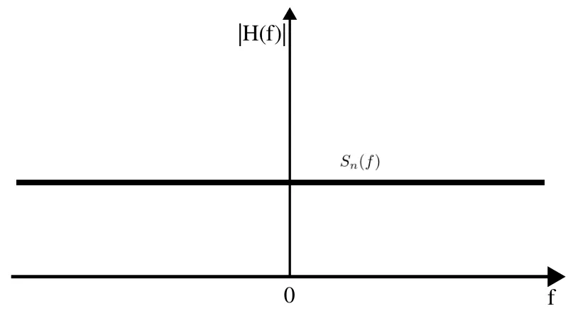
When white noise is the main source of issues, we can often improve circuit performance by adding simple filtering components to our system. This is where low-pass filters come in.

Low-Pass Filters(LPF)

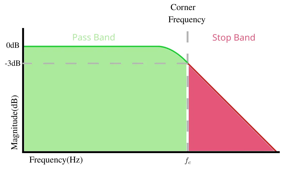
A low-pass filter refers to a filter that allows for low frequencies to "pass" meaning that they are not significantly attenuated (and typically not amplified). Along this, these filters also remove high frequency components by significantly attenuating them. This is what the frequency response of it looks like:

Screenshot_20251001_225757

There are many, many ways to design low-pass filters. In the case of labs we always want to design them in the simplest way possible, both in the number of components and in the way they are implemented into our system. For this reason we look to the RC circuit. There are 2 types of filters that we can make with these 2 components. A low-pass and a high-pass filter. We will only discuss low-pass filter design in this post.

RC LPF Theory

Screenshot_20251002_112425

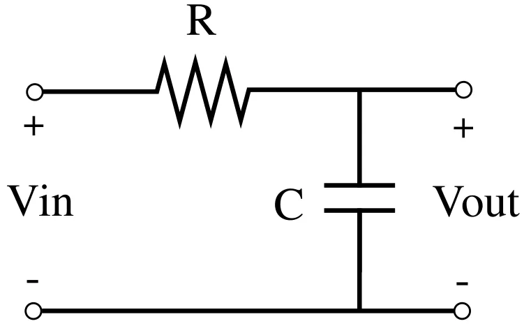
This is the simplest design of a low-pass filter. It is a resistor that connects 2 points followed by capacitor that connects from the output node to ground.

To understand why this forms a low-pass filter, we need to perform a brief analysis of this system.

A resistor's resistance is expressed as R, and the impedance of a capacitor is expressed as:

X_{c} = \frac{1}{j 2 π f C}

From this we can see that the impedance of this capacitor is inversely proportional to the frequency of the signals running through it. If we have 0 frequency (dc signal) then the capacitor will behave as an open circuit. If we have extremely high frequency (e.g. 10GHz) then the capacitor will behave as a short circuit.

The intuition of this comes from how a capacitor fundamentally works.

When a capacitor is fed to a power source the capacitor will charge until it becomes full, at which point it behaves like an open circuit. If we have a DC signal, we are permanently charging this capacitor without ever allowing it to discharge and thus it quickly fills and becomes open.

If we feed a signal that goes from positive to negative extremely fast, the capacitor will not have much time to actually hold on to the charge that goes through it because the signal will switch from charging to discharging too quickly. Thus charge does not build up and a capacitor acts like a wire, or a short circuit.

RC LPF Analysis

Let's analyze the RC circuit in the figure above. We know what the resistor's resistance is R, and the impedance of the capacitor is $X_{c} = \frac{1}{j 2 π f C}$ . We know what our input and output voltages are, and we can see that this setup forms a voltage divider. I will not show the derivation, but we can make this expression from the circuit:

V_{o} = V i (\frac{1}{1 + j 2 π f R C})

Testing our equation now, if we input the lowest frequency possible, we see that the term in the brackets will become $1 / 1$ and thus $V o = V i$ . Conversely if we have very high frequency, as we approach infinity, the term on the right will become $0$ . This then results in $V o = 0$ . In other words, our low frequencies pass, and our high frequencies are cut.

RC LPF Frequency Response

To get a more complete understanding of how to control an RC LPF, we need to understand the "corner frequency" parameter of the LPF transfer function. The corner frequency represents the "-3dB point" which refers to the point at which the output voltage is $0.707$ or $\frac{1}{\sqrt{2}}$ of the input voltage:

| \frac{V_{o u t}}{V_{i n}} | = \frac{1}{\sqrt{2}} \approx 0.707

If this seems a bit abstract, it may be helpful to think of the -3dB point as being the "half-power" point, the point at which our output power is half that of the input. If you are not interested in this, or already have a good understanding, you can skip to the next part by clicking here:

When looking at our Gain in dB, we have our formula of

G a i n (d B) = 10 \log (\frac{P_{o u t}}{P_{i n}})

Since we're looking for the half-power point, we can substitute $P_{o u t} = \frac{1}{2} P i n$ which makes our expression:

G a i n (d B) = 10 \log (\frac{1}{2})

This evaluates to $G a i n \approx - 3.01 d B$ . This is where the -3dB figure comes from. We, however, are not working with power measurements in our analysis. We work with voltage measurements, which means that the half-power equivalent value for voltage will be different. Our equation to solve for this is altered to accommodate $P \propto V^{2}$ :

G a i n (d B) = 10 \log (\frac{V_{o u t}^{2}}{V_{i n}^{2}})

Simplifying:

G a i n (d B) = 20 \log (\frac{V_{o u t}}{V_{i n}})

We want to see what value $\frac{V_{o u t}}{V_{i n}}$ must equal to when the system is at half-power, or -3dB. Our equation then follows:

20 \log (\frac{V_{o u t}}{V_{i n}}) = - 3

Solving:

\frac{V_{o u t}}{V_{i n}} = 10^{\frac{- 3}{20}} \approx 0.707 \approx \frac{1}{\sqrt{2}}

Continued...

First we find the magnitude of the expression we have:

V_{o} = V i (\frac{1}{1 + j 2 π f R C})

| \frac{V_{o}}{V_{i}} | = \frac{1}{\sqrt{1 + (2 π f R C)^{2}}}

| \frac{V_{o}}{V_{i}} | = \frac{1}{\sqrt{2}}

\frac{1}{\sqrt{1 + (2 π f_{c} R C)^{2}}} = \frac{1}{\sqrt{2}}

f_{c} = \frac{1}{2 π R C}

Now having a way to calculate the corner frequency it is now very simple to design LPFs that have certain cut off frequencies and pass bands.

Capacitors

In the lab kits used in all of the lab sections I've been a part of, there are always 2 types of capacitors in the kits. There are ceramic caps, and electrolytic caps.

Ceramic

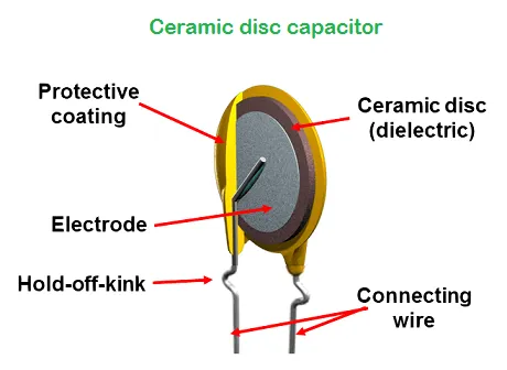
Ceramic capacitors are identifiable by their typical flattened shape when in TH mounting types along usually colorful protective coatings. These capacitors are as simple as it gets, being made up of 2 electrodes and a dielectric ceramic material. They are the easiest to use as they are bidirectional.

Electrolytic

Electrolytic capacitors are bulky and thick cylinders covered by typically black or blue plastic. These are not bidirectional, they have a + and - end that must be connected properly, or else it can lead to the capacitor being damaged or exploding. This is because of the way in which these are manufactured and what is inside them, I don't think this is important for this post.

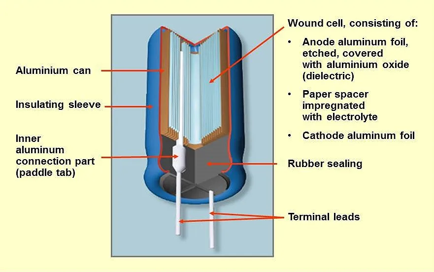
One of the most important details of capacitors that is never really introduced to students, is the notion that an electrolytic and a ceramic capacitor that both have the same capacitance value can have dramatically different performances.

Circuit analysis taught in classes deals with ideal capacitors and students never get the chance to develop an understanding for the important nuance of different types of capacitors.

Real capacitors have unwanted resistance and inductance introduced by their non-ideal forming materials and processes. For example, in an electrolytic capacitor, the leads of the capacitor will have non-zero resistance and inductance that is not usually considered.

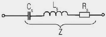
This is a more accurate model of a fabricated capacitor. There is some equivalent series inductance(ESL), and some equivalent series resistance(ESR). Typically ceramic capacitors will have lower ESL and ESR values even when comparing TH capacitors. It should be noted, however, that the difference in ESL and ESR is most stark when comparing TH electrolytic capacitors and SMD ceramic capacitors. Here is an impedance curve showing this difference:

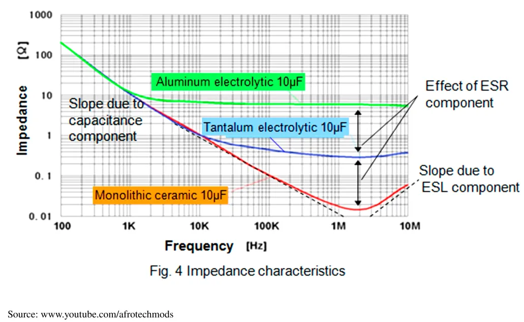
With that being said it is very much possible for there can be cases where the difference between the TH electrolytic and the TH ceramic actually do result in different and impactful circuit performance. Because of this it can be useful to play around with different capacitor types and capacitor combinations when tackling noise problems in lab circuits.

Visualizing Noise Filtering

To end this introduction I wanted to show a simple demonstration on how a signal can change by having white noise added to it, and by then adding filtering to make it more ideal. This was done using a PHET simulation linked here.

Let's say my input signal has a magnitude of 1.3 and a frequency of A3:

Screenshot_20251002_150450

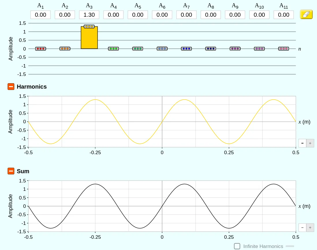
If I then add white noise, this is what my output wave will look like:

Screenshot_20251002_144648

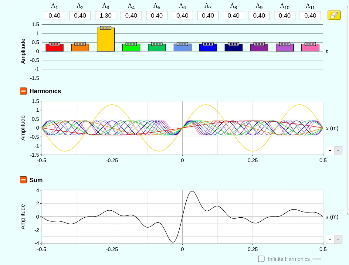
It's clear to see how distorted my wave becomes and how this signal would become likely unusable. But if we then replicate the effects of a LPF and cut off the higher end frequencies while only keeping the input signal and our low frequency noise...

Screenshot_20251002_144739

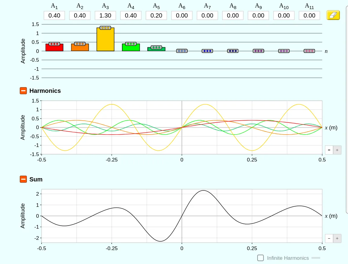
We can see a vast improvement by the introduction of a LPF.

I hope this post is useful in providing an understanding of the basics of filtering and the practical applications of it in a typical university lab setting. Though the focus was on low pass filters specifically, the fundamental ideas discussed here should be enough to guide similar analysis of high-pass filters.

FranciscoBragaResume

test